
Data Augmentation for Bias Term
Adding a constant feature folds the intercept into linear regression’s weight vector without conflating it with statistical bias.
Data Augmentation and the Bias Term
Observe the red highlighted in red.
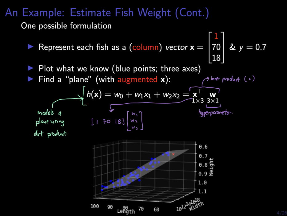
The ‘1’ is not the bias itself, but it’s a clever trick—often called data augmentation or adding a bias feature—that allows the bias term to be handled neatly for computational convenience.
Here’s the breakdown:
The Goal: A Linear Model
The goal is to estimate the fish’s weight () using its features (like length and girth ). A simple linear model for this looks like:
- and are the weights for each feature.
- is the bias or intercept. Geometrically, it’s the value of when all features are zero. It allows the prediction plane (the gray surface in your image) to be shifted up or down to better fit the data.
This equation involves a vector multiplication and a separate addition, which can be a bit clumsy.
The Trick: Combining Weights and Bias ✨
To simplify the computation, we can combine the bias term into the main weight vector.
Augment the Feature Vector (): We add a ‘1’ to the beginning of every feature vector.
- Original vector:
- Augmented vector:
Augment the Weight Vector (): We add the bias term to the beginning of our weight vector.
- Original vector:
- Augmented vector:
Now, let’s see what happens when we compute the dot product of these new, augmented vectors:
This gives us our original equation, , but now it’s expressed as a single, clean dot product operation.
Summary: Why Do This?
- Is it the bias? No, the ‘1’ is a constant feature. The weight that gets multiplied by this ‘1’ during the dot product becomes the model’s bias term.
- Is it to aid computation? Yes, absolutely. It simplifies the model’s representation from to a single operation . This is more elegant and efficient for both mathematical derivations and programming in machine learning libraries.
Bias Term vs Statistical Bias
Excellent question. The two terms sound similar but refer to very different concepts in machine learning.
The bias term is a part of your model, while actual bias (or statistical bias) is a way to describe how your model is wrong.
Bias Term (The Intercept)
The bias term ( or ) is a learnable parameter in models like linear and logistic regression. It’s simply the intercept of the model.
Its job is to allow the model to fit the data better. Without a bias term, a linear regression model would always have to pass through the origin (0,0), which is a huge and often incorrect limitation. The bias term allows the line or plane to be shifted up or down to find the best fit for the data.
💡 Think of it like this: Imagine you’re trying to draw a line through a cluster of data points. The weights determine the slope of the line, while the bias term determines where the line crosses the y-axis. You need both to position the line correctly.
Actual Bias (The Error)
Actual bias, often just called “bias” in the context of the bias-variance tradeoff, is a type of prediction error. It represents the difference between your model’s average prediction and the correct value you are trying to predict.
High bias means your model is making overly simple assumptions about the data. This causes the model to underfit—it fails to capture the underlying patterns. For example, trying to model a complex, curvy relationship with a simple straight line will result in high bias. The model is “biased” towards being a straight line and therefore can’t capture the true shape of the data.
The Key Difference
| Bias Term | Actual Bias (Statistical Bias) |
|---|---|
| What it is: A parameter in the model (the intercept). | What it is: A type of prediction error. |
| Purpose: To give the model more flexibility. | Meaning: It indicates the model is too simple (underfitting). |
| How you get it: The model learns it during training. | How you get it: It arises from incorrect model assumptions. |
| Is it bad? No, it’s a necessary and helpful part of the model. | Is it bad? Yes, high bias is a sign of a poor model fit. |
The bias term allows a model to learn an offset, providing more flexibility to fit the data. Think of it as the y-intercept in the classic line equation, .
Why is a Bias Term Needed?
Without a bias term, a linear model’s line is forced to pass through the origin (0, 0). This is a major restriction because most real-world data doesn’t start at the origin. The bias term b allows the line to be shifted up or down to better fit the data points.
Example: Predicting Weight from Height
Imagine we have data for people’s heights and weights. A person with zero height should have zero weight, so you might think a line through the origin works. But the data might look like this:
- Red Line (No Bias): The model is forced through (0,0). It clearly misses the trend in the data.
- Green Line (With Bias): The model can shift vertically. The bias term
ballows the line to start from a more realistic point, providing a much better fit.
How the Column of Ones Creates the Bias
The goal in machine learning is to express our model in a clean, efficient matrix multiplication:
Here, are the predictions, is the input data, and is the vector of weights (parameters) the model learns.
Let’s see how adding a column of ones makes this work.
Case 1: Without the Bias Column
Suppose we have two data points and one feature (e.g., height). Our equation is just .
Input matrix (2 points, 1 feature):
Weight vector (1 weight):
The matrix multiplication gives:
Notice there’s no way to add a separate bias term b.
Case 2: With the Bias Column (Augmented Input)
Now, we add a column of ones to . The model we want is . We can cleverly rename the bias to and say the full equation is , where is always 1.
Augmented input matrix (the
1is the added bias feature):Weight vector (now has 2 weights, one for bias
w_0and one for the featurew_1):Now, let’s do the matrix multiplication :
Success! 🎉 By adding that column of ones, the weight that gets learned by the model acts exactly like the bias term b. This trick allows us to handle both the feature weights and the bias in a single, elegant matrix operation.